Building an AI Financial Market Model - Lesson I
Part 1
Before you can begin with building your own AI Financial Market Model (machine learned), you have to decide on what software to use. Since I wrote this article in 2007, many new advances have been made in machine learning. Notably the python module Scikit Learn came out and Hadoop was released into the wild.
I’m not overly skilled in coding and programming — I know enough to get by- I settled on RapidMiner. RapidMiner is a very simple visual programming platform that let’s you drag and drop “operators” into a design canvas. Each operator has a specific type of task related to ETL, modeling, scoring, and extending the features of RapidMiner.
There is a slight learning curve but, it’s not hard to learn if you follow along with this tutorial!
The AI Financial Market Model
First download RapidMiner Studio and then get your market data (OHLCV prices), merge them together, transform the dates, figure out the trends, and so forth. Originally these tutorials built a simple classification type of model that look to see if your trend was classified as being in an “up-trend” or a “down-trend.” The fallacy was they didn’t not take into account the time series nature of the market data and the resulting model was pretty bad.
For this revised tutorial we’re going to do a few things.
- Install the Finance and Economics, and Series Extensions
- Select the S&P500 weekly OHLCV data for a range of 5 years. We’ll visualize the closing prices and auto-generate a trend label (i.e. Up or Down)
- We’ll add in other market securities (i.e. Gold, Bonds, etc) and see if we can do some feature selection
- Then we’ll build a forecasting model using some of new H20.ai algorithms included in RapidMiner v7.2
All processes will be shared and included in these tutorials. I welcome your feedback and comments.
The Data
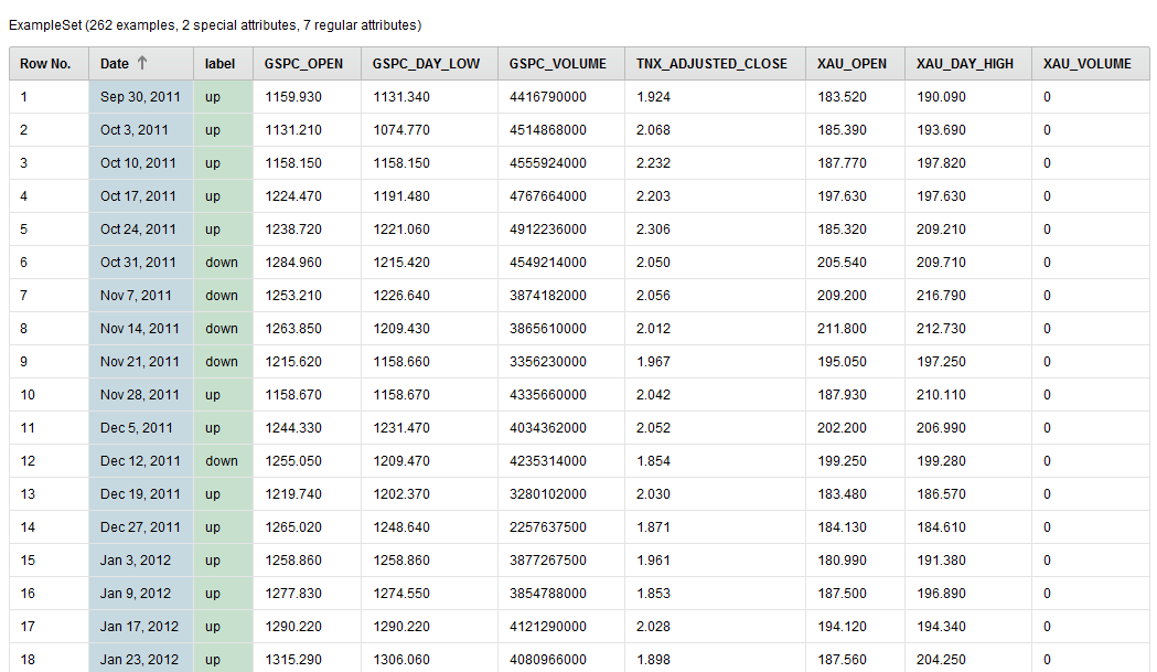
We’re going to use the adjusted closing prices of the S&P500, 10 Year Bond Yield, and the Philadelphia Gold Index from September 30, 2011 through September 20, 2016.
The raw data looks like this:
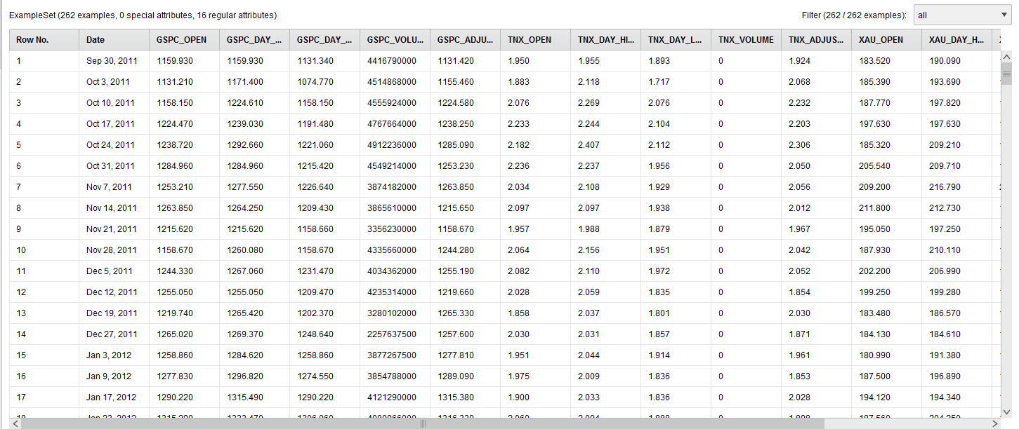 RapidMiner AI Raw Data
We renamed the columns (attributes) humanely by removing the “^” character from the stock symbols.
Next we visualized the adjusted weekly closing price of the S&P500 using the built in visualization tools of RapidMiner.
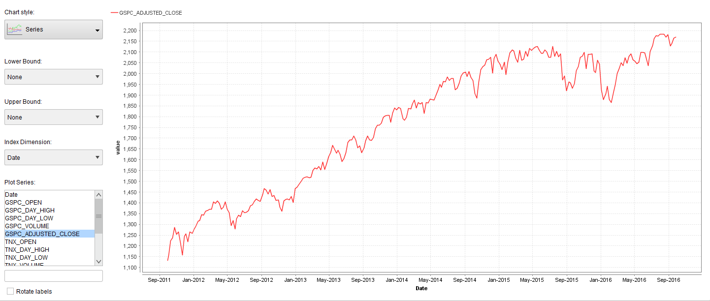 RapidMiner AI Time Series
The next step will be to transform the S&P500 adjusted closing price into Up and Down trend labels. To automatically do this we have to install the RapidMiner Series Extension and use the Classify by Trend operator. The Classify by Trend operator can only work if you set the set the SP500_Adjusted_Close column (attribute) as a Label role.
The Label role in RapidMiner is your target variable. In RapidMiner all data columns come in as “Regular” roles and a “Label” role is considered a special role. It’s special in the sense that it’s what you want the machine learned model to learn to. To achieve this you’ll use the Set Role operator. In the sample process I share below I also set the Date to the ID role. The ID role is just like a primary key, it’s useful when looking up records but doesn’t get built into the model.
The final data transformation looks like this:
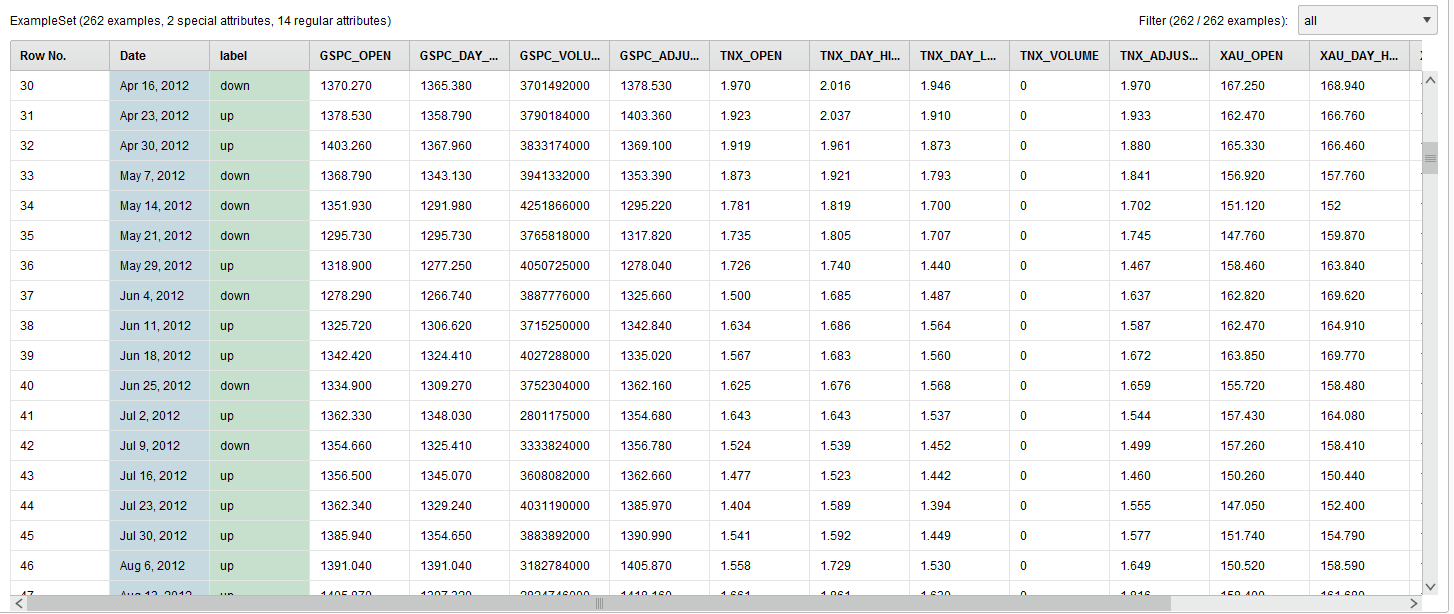 RapidMiner AI Time Series Transformed
The GSPC_Adjusted_Close column is now transformed and renamed to the label column.
The resulting process looks like this:
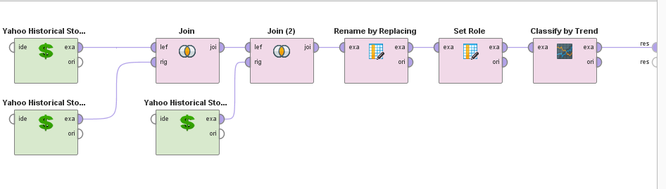 RapidMiner AI Time Series Process
Part 2
In Part 2 I want to show you how to use MultiObjective Feature Selection (MOFS) in RapidMiner. It’s a great technique to simultaneously reduce your attribute set and maximize your performance (hence: MultiObjective). This feature selection process can be run over and over again for your AI Financial Market Model, should it begin to drift.
Load in the Process From Tutorial One
At the bottom of that post you can download the RapidMiner process.
Add an Optimize Selection (Evolutionary) Operator
The data that we pass through the process contains the adjusted closing prices of the S&P500, 10 Year Bond Yield, and the Philadelphia Gold. Feature Selection let’s us chose which one of these attributes contributes the most to the overall model performance, and which really don’t matter at all.
To do that, we need to add an Optimize Selection (Evolutionary) operator.
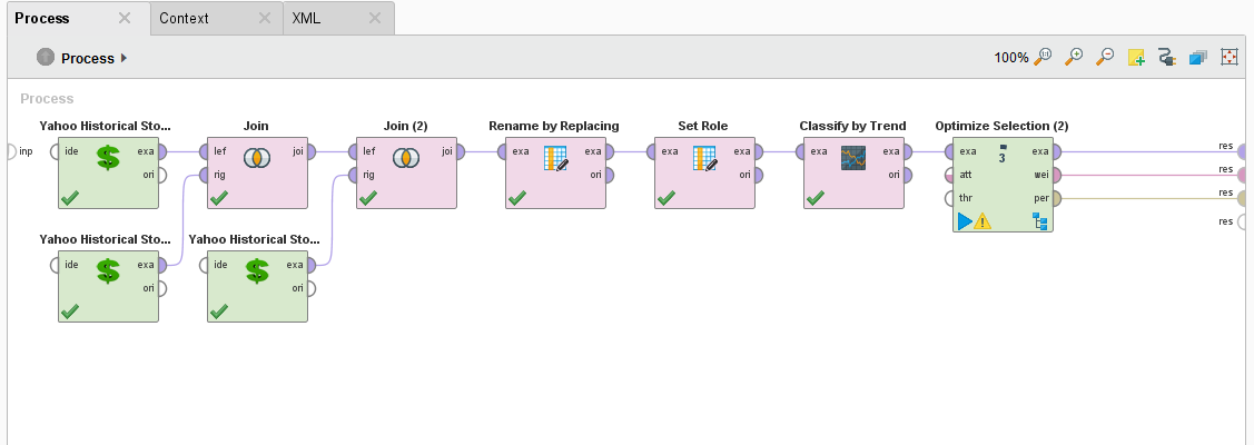 RapidMiner AI Process
Why do you want to do MultiObjective Feature Selection? There are many reasons but most important of all is that a smaller data set increases your training time by reducing consumption of your computer resources.
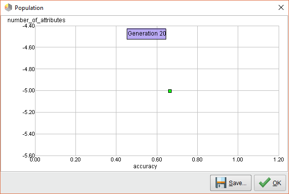
When we execute this process, you can see that the Optimize Selection (Evolutionary) operator starts evaluating each attribute. At first, it measures the performance of ALL attributes and it looks like it’s all over the map.
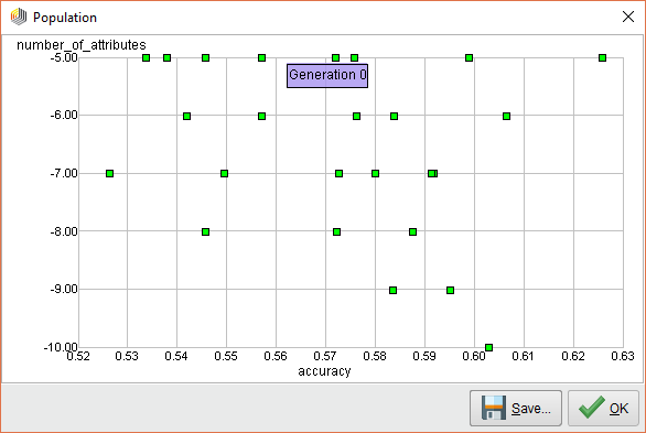 RapidMiner AI Feature Generation 0
How it measures the performance is with a Cross Validation operator embedded inside the subprocess.
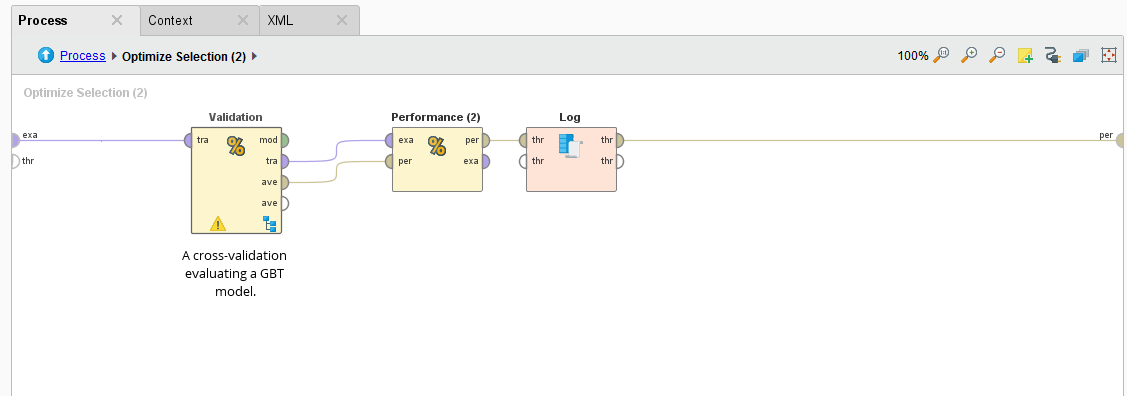 RapidMiner Cross Validation
The Cross Validation operator use a Gradient Boosted Tree algorithm to analyze the permutated inputs and measures their performance in an iterative manner. Attributes are removed if they don’t provide an increase in performance.
MultiObjective Feature Selection Results
From running this process, we see that the following attributes provide the best performance over 25 iterations.
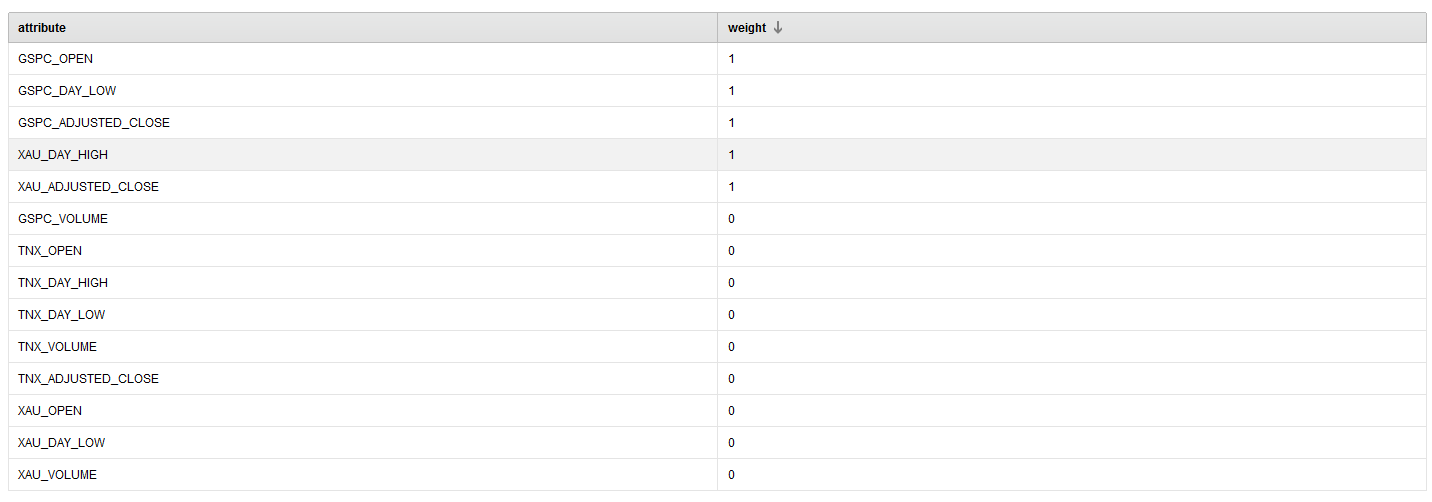 RapidMiner Selected Features
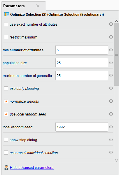 Hyperparameters
Note: We choose to have a minimum of 5 attributes returned in the parameter configuration. The selected ones have a weight of 1.
The resulting performance for this work is below.
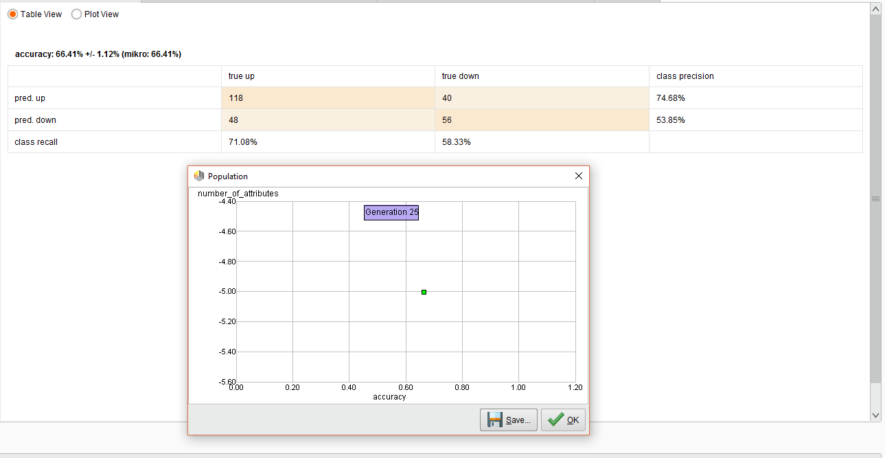 Experiment Performance
The overall accuracy was 66%. In the end predicting and UP trend was pretty decent, but not so good for the DOWN trend.
The possible reason for this poor performance is that I purposely made a mistake here. I used a Cross Validation operator instead of using a Sliding Window Validation operator.
The Sliding Window Validation operator is used to backtest and train a time series model in RapidMiner and we’ll explain the concepts of Windowing and Sliding Window Validation in the next Lesson.
Note: You can use the above method of MultiObjective Feature Selection for both time series and standard classification tasks.
Part 3
In Part 2 I went over the concept of MultiObjective Feature Selection (MOFS). In this lesson we’ll build on MOFS for our model but we’ll forecast the trend and measure it’s accuracy.
Revisiting Mofs
We learned in lesson 2 that RapidMiner can simultaneously select the best features in your data set while maximizing the performance. We ran the process and the best features were selected below.
 MultiObjective Feature Selection
From here we want to feed the data into three new operators that are part of the Series Extension. We will be using the Windowing, Sliding Window Validation, and the Forecasting Performance operator.
These there operators are key to measure a performance of your time series model. RapidMiner is really good and determining the directional accuracy of time series and a bit rough when it comes to point forecasts. My personal observation is that it’s futile to get a point forecast for an asset price, you have better luck with direction and volatility.
Our forecasting model will use a Support Vector Machine and and RBF kernel. Time series appear to benefit from this combination and you can always check out this link for more info.
Forecast Trend Accuracy
 Forecast Trend Accuracy
The Process
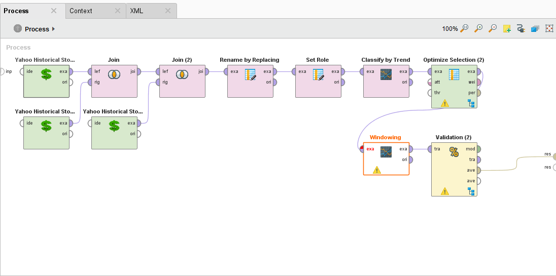 Forecast Trend Accuracy Process
Sliding Window Validation Parameters
 Sliding Window Parameters
Windowing the Data
RapidMiner allows you to do multivariate time series analysis also known as a model driven approach to analysis. This is different than a data driven approach, such as ARIMA, and allows you to use many different inputs to make a forecast. Of course, this means that point forecasting becomes very difficult when you have multiple inputs, but makes directional forecast more robust.
The model driven approach in RapidMiner requires you to Window your Data. To do that you’ll need to use the Window operator. This operator is often misunderstood, so I suggest you read my post in the community on how it works.
Tip: Another great reference on using RapidMiner for time series is here.
There are key parameters that you should be aware of especially the window size, the step size, whether or not you create a label, and the horizon.
 Optimization parameters
When it comes to time series for the stock market, I usually choose a value of 5 for my window. This can be fore 5 days, if your data is daily, or 5 weeks if it’s weekly. You can choose what you think is best.
The Step Size parameter tells the Windowing operator to create a new window with the next example row it encounters. If it was set to two, then it will move two examples ahead and make a new window.
Tip: The Series Representation parameter is defaulted to “encode_series_by_examples.” You should leave this default if your time series data is row by row. If a new value of your time series data is in a new column (e.g. many columns and one row), then you should change it to “encode_series_by_attributes.”
Sliding Validation
The Sliding Window Validation operator is what is used to backtest your time series, it operates differently than a Cross Validation because it creates a “time window” on your data, builds a model, and tests it’s performance before sliding to another time point in your time series.
Sliding Window Parameters
In our example we create a training and testing window width of 10 example rows, our step size is -1 (which is the size of the last testing window), and our horizon is 1. The horizon is how far into the future we want to predict, in this case it’s 1 example row.
There are some other interesting toggle parameters to choose from. The default is average performances only, so your Forecast Trend Accuracy will be your average performance. If you toggle on “cumulative training” then the Sliding Window Validation operator will keep adding the previous window to the training set. This is handy if you want see if the past time series data might affect your performance going forward BUT it makes training and testing very memory intensive.
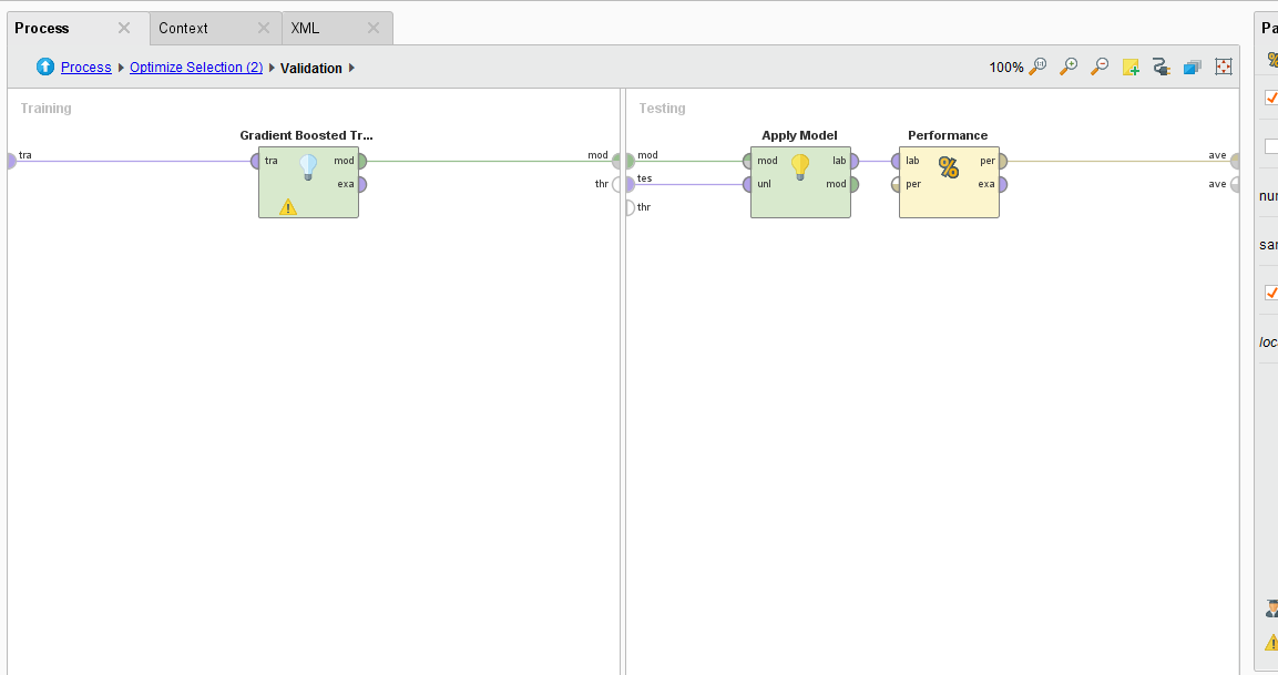
Double clicking on the Sliding Window Validation operator we see a typical RapidMiner Validation training and testing sides where we can embed our SVM, Apply Model, and Forecasting Performance operators. The Forecasting Performance operator is a special Series Extension operator. You need to use this to forecast the trend on any time series problem.
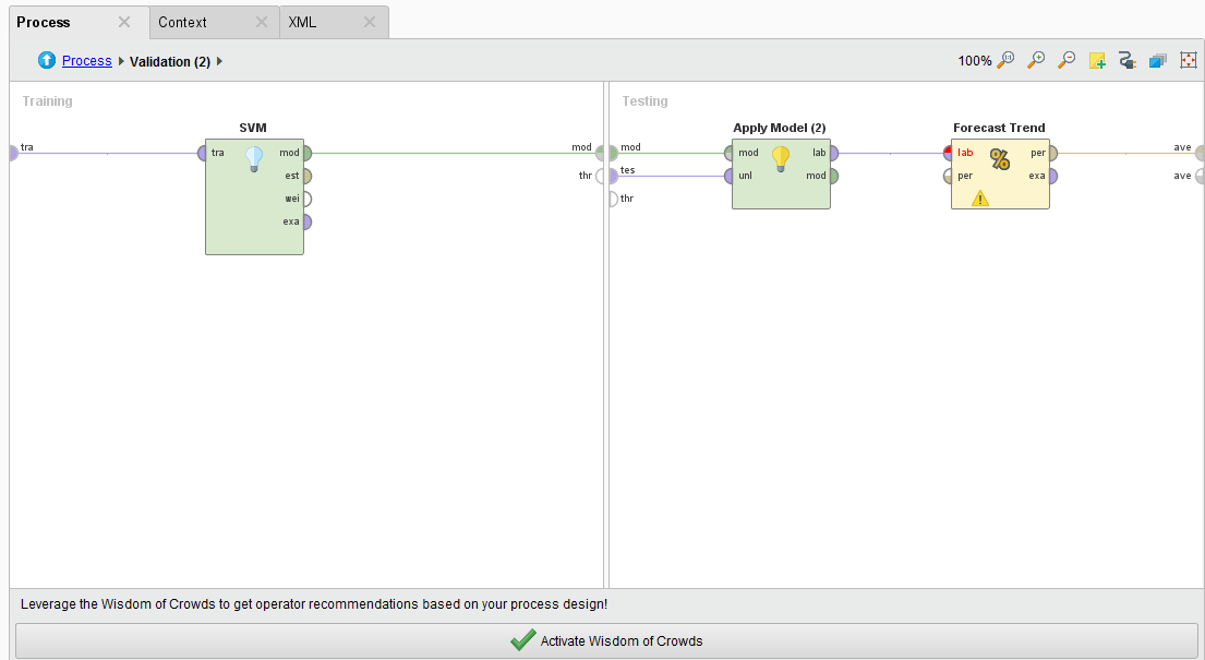 Sliding Window Guts
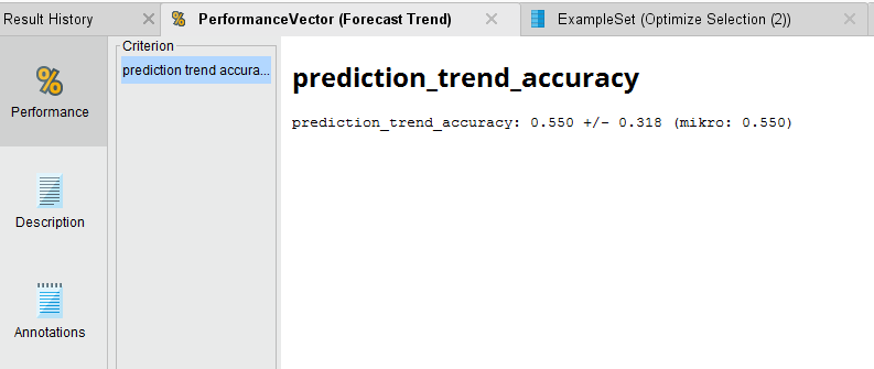
Forecast the Trend
Once we run the process and the analysis completes, we see that we have a 55.5% average accuracy to predict the direction of the trend. Not great, but we can see if we can optimize the SVM parameters of C and gamma to get better performance out of the model.
 Forecast Trend Accuracy
In my next lesson I’ll go over how to do Optimization in RapidMiner to better forecast the trend.
Part 4
In Part 3, I introduced the Sliding Window Validation operator to test how well we can forecast a trend in a time series. Our initial results are very poor, we were able to forecast the trend with an average accuracy of 55.5%. This is fractionally better than a simple coin flip! In this updated lesson I will introduce the ability of Parameter Optimization in RapidMiner to see if we can forecast the trend better.
Parameter Optimization
We begin with the same process in Lesson 3 but we introduce a new operator called the Optimize Parameter (Grid) operator. We also do some house cleaning for putting this process into production.
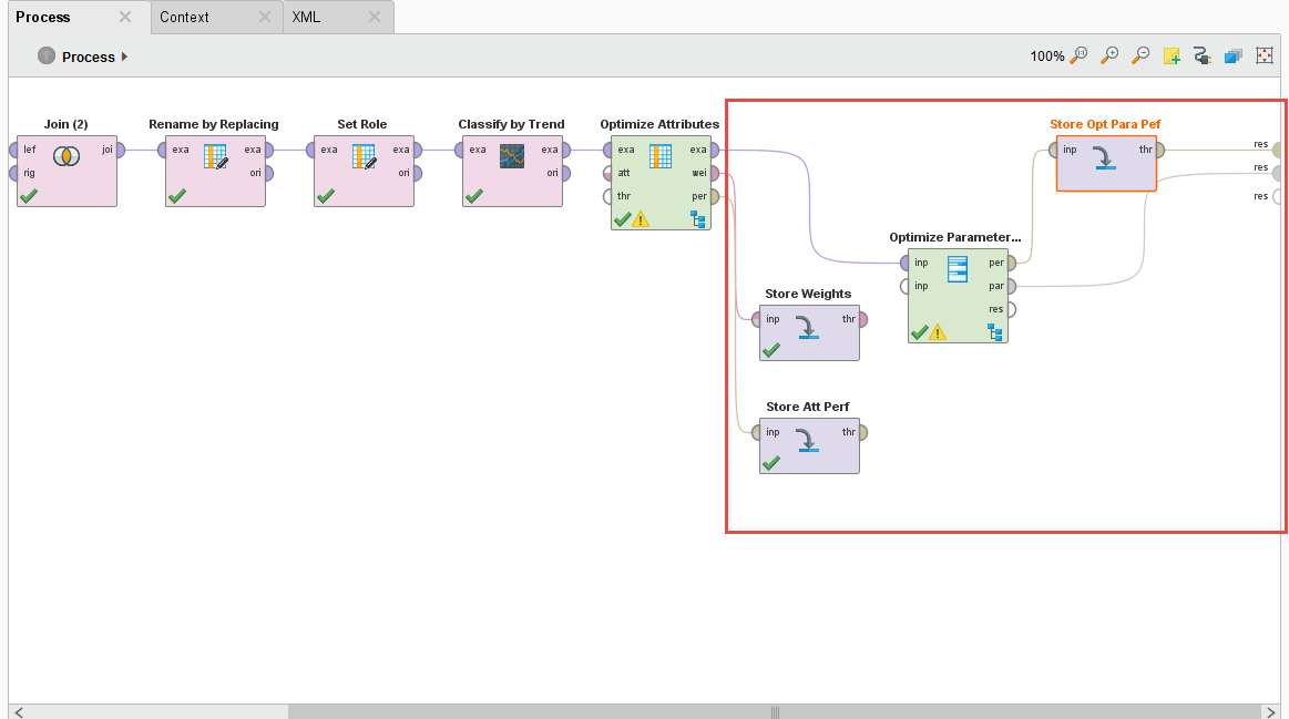 RapidMiner Finance AI model proess
The Optimize Parameter (Grid) operator let’s you do some amazing things, it lets you vary — by your predefined limits — parameter values of different operators. Any operator that you put inside this operator’s subprocess can have their parameters automatically iterated over and the overall performance measured. This is a great way to fine tune and optimize models for your analysis and ultimately for production.
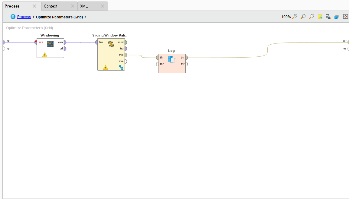 Inside the Optimize Parameters Option
For our process, we want to vary the training window width, testing window width, training step width on the Sliding Window Validation operator, the C and gamma parameter of the SVM machine learning algorithm, and the forecasting horizon on the Forecast Trend Performance operator. We want to test all combinations and ultimately determine the best combination of these parameters that will give us the best tuned trend prediction.
Note: I run a weekly optimization process for my volatility trend predictions. I’ve noticed depending on market activity, the training width of the Sliding Window Validation operator needs to be tweaked between 8 and 12 weeks.
I also add a few Store operators to save the Performance and Weights of the Optimize Selection operator, and the Performance and Parameter Set of the Optimization Parameter (Grid) operator. We’ll need this data for production.
Varying Parameters Automatically
Whatever operators you put inside the Optimize Parameters (Grid) operator can have their parameters varied automatically, you just have to select which ones and set minimum and maximum values. Just click on the Edit Parameter settings button. Once you do, you are presented with a list of available operators to vary. Select one operator and another list of available parameters is shown. Then select which parameter you want and define min/max values.
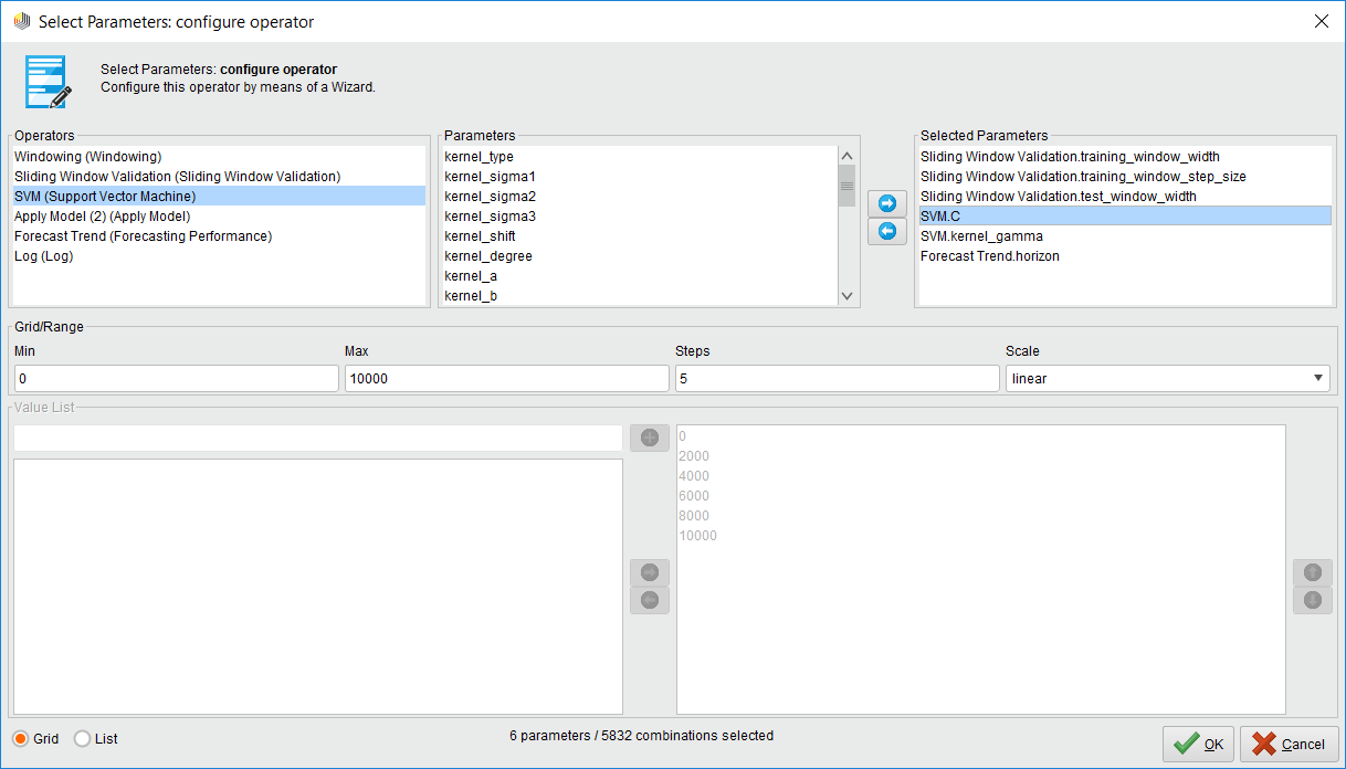 Inside the Optimize Parameters Option Part 2
Note: If you select a lot of parameters to vary with a very large max value, you could be optimizing for hours and even days. This operator consumes your computer resources when you millions of combinations!
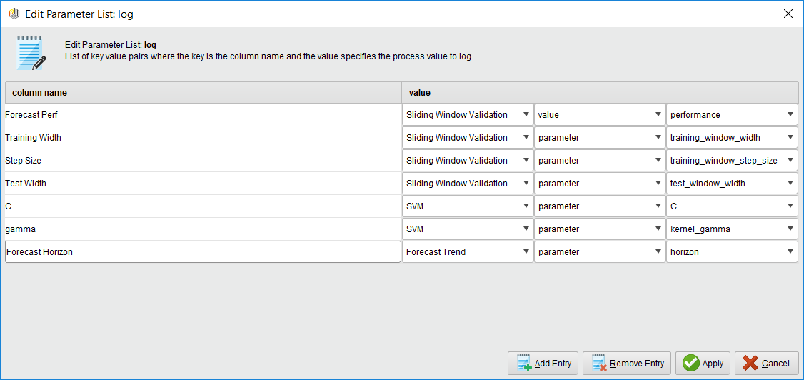
The Log File
The log file is a handy operator that we use in optimization because we can create a custom log file that has the values of the parameters we’re measuring and the resulting forecast performance. You just name your column and select which operator and parameter you want to have an entry for.
 The handy Log Operator
Pro Tip: If you want to measure the performance, make sure you select the Sliding Window Validation operator’s performance port and NOT the Forecast Trend Performance operator. Why? Because the Forecast Trend Performance operator generates several models as it slides across the time series. Some performances are better than others. The Sliding Window Validation operator averages all the results together, and that’s the measure you want!
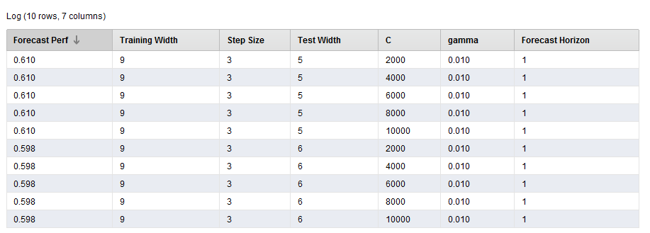 Log Operator Part 2
This is a great way of seeing what initial parameter combinations are generating the best performance. It can also be used to visualize your best parameter combinations too!
The Results
The results are point to a parameter combination of:
- Training Window Width: 10
- Testing Window Width: 5
- Step Width: 4
- C: 0
- Gamma: 0.1
- Horizon: 3
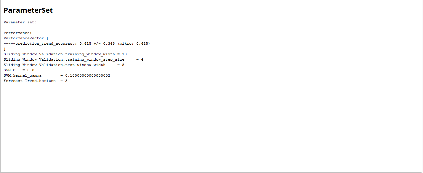 Setting RapidMiner Parameters
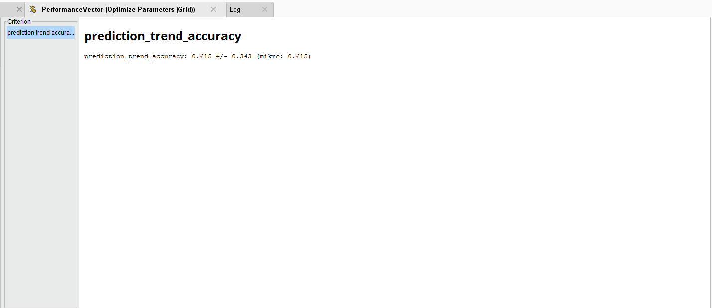 Optimizing Trend Accuracy
To generate an average Forecast Trend accuracy of 61.5%. Compared to the original accuracy, this is an improvement.
End Notes
There you have it, all four parts (lessons) on how to build a RapidMiner AI finance model without coding.